



















• bitcoinBitcoin(BTC)$77,428.000.02%
  • ethereumEthereum(ETH)$2,248.600.48%
  • tetherTether(USDT)$1.000.01%
  • binancecoinBNB(BNB)$704.950.75%
  • rippleXRP(XRP)$1.250.13%
  • usd-coinUSDC(USDC)$1.000.02%
  • solanaSolana(SOL)$95.74-0.85%
  • tronTRON(TRX)$0.320521-5.89%
  • Figure HelocFigure Heloc(FIGR_HELOC)$1.030.00%
  • zcashZcash(ZEC)$1,281.992.70%
  • HyperliquidHyperliquid(HYPE)$88.14-4.55%
  • dogecoinDogecoin(DOGE)$0.075174-0.55%
  • moneroMonero(XMR)$595.580.45%
  • USDSUSDS(USDS)$1.000.02%
  • chainlinkChainlink(LINK)$11.534.26%
  • whitebitWhiteBIT Coin(WBT)$74.370.22%
  • leo-tokenLEO Token(LEO)$9.38-0.51%
  • cardanoCardano(ADA)$0.192587-0.36%
  • stellarStellar(XLM)$0.1688562.06%
  • bitcoin-cashBitcoin Cash(BCH)$290.472.33%
  • nearNEAR Protocol(NEAR)$4.330.37%
  • daiDai(DAI)$1.000.03%
  • Ethena USDeEthena USDe(USDE)$1.00-0.01%
  • RainRain(RAIN)$0.006138-7.91%
  • uniswapUniswap(UNI)$6.951.29%
  • litecoinLitecoin(LTC)$54.89-0.75%
  • USD1USD1(USD1)$1.00-0.01%
  • CantonCanton(CC)$0.0960710.64%
  • avalanche-2Avalanche(AVAX)$8.44-1.10%
  • suiSui(SUI)$0.901.22%
  • the-open-networkGram (prev. Toncoin)(GRAM)$1.180.46%
  • hedera-hashgraphHedera(HBAR)$0.0722890.29%
  • tether-goldTether Gold(XAUT)$3,874.57-2.35%
  • Global DollarGlobal Dollar(USDG)$1.00-0.03%
  • quant-networkQuant(QNT)$196.721.98%
  • paypal-usdPayPal USD(PYUSD)$1.000.01%
  • shiba-inuShiba Inu(SHIB)$0.000005-0.75%
  • BittensorBittensor(TAO)$235.370.93%
  • crypto-com-chainCronos(CRO)$0.051417-1.16%
  • EthenaEthena(ENA)$0.1909132.47%
  • Ripple USDRipple USD(RLUSD)$1.00-0.02%
  • Ondo US Dollar YieldOndo US Dollar Yield(USDY)$1.15-0.10%
  • Circle USYCCircle USYC(USYC)$1.140.03%
  • okbOKB(OKB)$110.74-0.50%
  • MemeCoreMemeCore(M)$0.95-4.87%
  • pepePepe(PEPE)$0.000005-3.25%
  • aaveAave(AAVE)$133.786.82%
  • BlackRock USD Institutional Digital Liquidity FundBlackRock USD Institutional Digital Liquidity Fund(BUIDL)$1.000.00%
  • OndoOndo(ONDO)$0.4078644.38%
  • Pump.funPump.fun(PUMP)$0.0041190.95%
TradePoint.io
  • Main
  • AI & Technology
  • Stock Charts
  • Market & News
  • Business
  • Finance Tips
  • Trade Tube
  • Blog
  • Shop
No Result
View All Result
TradePoint.io
No Result
View All Result

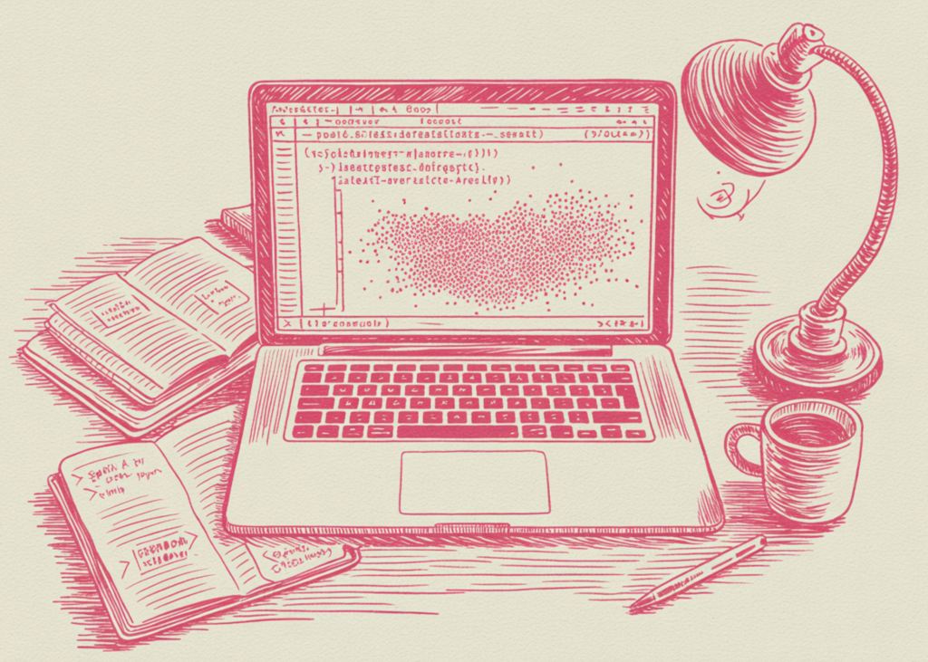
A Coding Tutorial on Datashader on Rendering Massive Datasets with High-Performance Python Visual Analytics

April 26, 2026
in AI & Technology
Reading Time: 3 mins read
A A
A Coding Tutorial on Datashader on Rendering Massive Datasets with High-Performance Python Visual Analytics
ShareShareShareShareShare
import subprocess, sys
subprocess.check_call([sys.executable, "-m", "pip", "install", "-q",
                      "datashader", "colorcet", "numba", "scipy"])


import numpy  as np
import pandas as pd
import datashader as ds
import datashader.transfer_functions as tf
from datashader import reductions as rd
import colorcet as cc
import matplotlib.pyplot as plt
import matplotlib.colors as mcolors
from matplotlib.gridspec import GridSpec
from scipy.stats import multivariate_normal
import time, warnings
warnings.filterwarnings("ignore")


print("Datashader version:", ds.__version__)


def show(img, title="", ax=None, figsize=(6, 5)):
   standalone = ax is None
   if standalone:
       fig, ax = plt.subplots(figsize=figsize)
   rgba = img.to_pil()
   ax.imshow(rgba, origin="upper", aspect="auto")
   ax.set_title(title, fontsize=11, fontweight="bold")
   ax.axis("off")
   if standalone:
       plt.tight_layout()
       plt.show()


print("\n=== SECTION 1: Core Pipeline ===")


rng = np.random.default_rng(42)
N   = 2_000_000


x = np.concatenate([rng.normal(-1, 0.5, N//3),
                   rng.normal( 1, 0.5, N//3),
                   rng.normal( 0, 1.5, N//3)])
y = np.concatenate([rng.normal(-1, 0.5, N//3),
                   rng.normal( 1, 0.5, N//3),
                   rng.normal( 0, 0.5, N//3)])
df_base = pd.DataFrame({"x": x, "y": y})


canvas = ds.Canvas(plot_width=600, plot_height=500,
                  x_range=(-4, 4), y_range=(-4, 4))


agg = canvas.points(df_base, "x", "y", agg=rd.count())


fig, axes = plt.subplots(1, 3, figsize=(15, 4))
combos = [
   ("Linear / blues",  tf.shade(agg, cmap=cc.blues,        how="linear")),
   ("Log    / fire",   tf.shade(agg, cmap=cc.fire,         how="log"   )),
   ("Eq-hist / bmy",   tf.shade(agg, cmap=cc.bmy,          how="eq_hist")),
]
for ax, (title, img) in zip(axes, combos):
   show(img, title, ax=ax)
plt.suptitle("Section 1 – 2 M points: Linear vs Log vs Eq-Hist normalisation",
            fontsize=13, fontweight="bold")
plt.tight_layout()
plt.show()


print("\n=== SECTION 2: Reduction Types ===")


n_actual = len(df_base)
df_base["value"] = rng.exponential(scale=2, size=n_actual)
df_base["label"] = pd.Categorical(
   rng.choice(["A", "B", "C"], size=n_actual),
   categories=["A", "B", "C"]
)


canvas2 = ds.Canvas(plot_width=400, plot_height=350,
                   x_range=(-4, 4), y_range=(-4, 4))


reductions_cfg = [
   ("count()",          rd.count(),                 cc.kbc),
   ("sum(value)",       rd.sum("value"),             cc.CET_L3),
   ("mean(value)",      rd.mean("value"),            cc.CET_D4),
   ("std(value)",       rd.std("value"),             cc.CET_L16),
   ("min(value)",       rd.min("value"),             cc.CET_L17),
   ("max(value)",       rd.max("value"),             cc.bgyw),
   ("var(value)",       rd.var("value"),             cc.CET_L18),
   ("count_cat(label)", rd.count_cat("label"),       None),
]


fig, axes = plt.subplots(2, 4, figsize=(18, 9))
axes = axes.flat


for ax, (name, agg_fn, cmap) in zip(axes, reductions_cfg):
   agg_r = canvas2.points(df_base, "x", "y", agg=agg_fn)
   if cmap is None:
       img = tf.shade(agg_r, color_key={"A":"#e41a1c","B":"#377eb8","C":"#4daf4a"})
   else:
       img = tf.shade(agg_r, cmap=cmap, how="eq_hist")
   show(img, name, ax=ax)


plt.suptitle("Section 2 – All Reduction Types on 2 M points", fontsize=14, fontweight="bold")
plt.tight_layout()
plt.show()


print("\n=== SECTION 3: Categorical Visualisation ===")


N_cat = 500_000
categories = ["Cluster A", "Cluster B", "Cluster C", "Cluster D"]
centers = [(-2, -2), (-2, 2), (2, -2), (2, 2)]
colors  = {"Cluster A":"#e41a1c","Cluster B":"#377eb8",
          "Cluster C":"#4daf4a","Cluster D":"#ff7f00"}


frames = []
for cat, (cx, cy) in zip(categories, centers):
   n = N_cat // len(categories)
   frames.append(pd.DataFrame({
       "x":    rng.normal(cx, 0.8, n),
       "y":    rng.normal(cy, 0.8, n),
       "cat":  pd.Categorical([cat]*n, categories=categories),
   }))
df_cat = pd.concat(frames, ignore_index=True)


canvas3 = ds.Canvas(plot_width=500, plot_height=500,
                   x_range=(-5, 5), y_range=(-5, 5))
agg_cat = canvas3.points(df_cat, "x", "y", agg=rd.count_cat("cat"))


fig, axes = plt.subplots(1, 3, figsize=(16, 5))


img_raw  = tf.shade(agg_cat, color_key=colors)
show(img_raw, "Raw (no spread)", ax=axes[0])


img_sp1  = tf.spread(tf.shade(agg_cat, color_key=colors), px=1)
show(img_sp1, "Spread px=1", ax=axes[1])


img_bg   = tf.set_background(tf.shade(agg_cat, color_key=colors), color="black")
show(img_bg, "Black background", ax=axes[2])


for cat, col in colors.items():
   axes[2].plot([], [], "o", color=col, label=cat, markersize=8)
axes[2].legend(loc="lower right", fontsize=8, framealpha=0.6)


plt.suptitle("Section 3 – Categorical Rendering (500 k points)", fontsize=13, fontweight="bold")
plt.tight_layout()
plt.show()

Credit: Source link

YOU MAY ALSO LIKE

Google Joins OpenAI And Anthropic In Promising New Scraping Controls

Apple Brings First Apple Intelligence Features to China in iOS 27.3 – Unite.AI

ShareTweetSendSharePin

Related Posts

Google Joins OpenAI And Anthropic In Promising New Scraping Controls
AI & Technology

Google Joins OpenAI And Anthropic In Promising New Scraping Controls

October 31, 2026
Apple Brings First Apple Intelligence Features to China in iOS 27.3 – Unite.AI
AI & Technology

Apple Brings First Apple Intelligence Features to China in iOS 27.3 – Unite.AI

October 30, 2026
Powerlattice Raises M in Equity Offering, SEC Filing Shows – Unite.AI
AI & Technology

Powerlattice Raises $86M in Equity Offering, SEC Filing Shows – Unite.AI

October 30, 2026
Databricks Expands SAP Partnership with Genie, Lakeflow, and Lakebase – Unite.AI
AI & Technology

Databricks Expands SAP Partnership with Genie, Lakeflow, and Lakebase – Unite.AI

October 30, 2026
Next Post
Shortage of critical specialty doctor impacts patients nationwide

Shortage of critical specialty doctor impacts patients nationwide

Leave a Reply Cancel reply

Your email address will not be published. Required fields are marked *

Search

No Result
View All Result
Current with Christine Romans – Oct. 13 | NBC News NOW

Current with Christine Romans – Oct. 13 | NBC News NOW

October 26, 2026
Current with Christine Romans – Oct. 15 | NBC News NOW

Current with Christine Romans – Oct. 15 | NBC News NOW

October 25, 2026
Bend school shooter identified as 16-year-old resident

Bend school shooter identified as 16-year-old resident

October 24, 2026

About

Learn more

Our Services

Legal

Privacy Policy

Terms of Use

Bloggers

Learn more

Article Links

Contact

Advertise

Ask us anything

©2020- TradePoint.io - All rights reserved!

Tradepoint.io, being just a publishing and technology platform, is not a registered broker-dealer or investment adviser. So we do not provide investment advice. Rather, brokerage services are provided to clients of Tradepoint.io by independent SEC-registered broker-dealers and members of FINRA/SIPC. Every form of investing carries some risk and past performance is not a guarantee of future results. “Tradepoint.io“, “Instant Investing” and “My Trading Tools” are registered trademarks of Apperbuild, LLC.

This website is operated by Apperbuild, LLC. We have no link to any brokerage firm and we do not provide investment advice. Every information and resource we provide is solely for the education of our readers. © 2020 Apperbuild, LLC. All rights reserved.

No Result
View All Result
  • Main
  • AI & Technology
  • Stock Charts
  • Market & News
  • Business
  • Finance Tips
  • Trade Tube
  • Blog
  • Shop

© 2023 - TradePoint.io - All Rights Reserved!