







































In this advanced QuTiP tutorial, we explore the rich dynamics of quantum systems using Python and the QuTiP framework. We’ll begin by preparing fundamental single- and two-qubit states, including Bell pairs, and then move on to implement key quantum operations such as Pauli matrices, Hadamard gates, and CNOT. From there, we’ll simulate Rabi oscillations in a driven two-level system, investigate coherent state evolution in a quantum harmonic oscillator, and model decoherence in open systems. We’ll visualize phase-space trajectories via Wigner functions and quantify entanglement generation between coupled qubits. By the end of this tutorial, you’ll have built a complete workflow for state preparation, time evolution, open-system dynamics, and entanglement analysis, all within a Colab environment. Check out the FULL CODES here.
!pip install qutip matplotlib numpy


import numpy as np
import matplotlib.pyplot as plt
from qutip import *


print("🔬 Advanced QuTip Tutorial: Quantum Dynamics & Entanglement")
print("=" * 60)
In the setup phase, we install QuTiP along with NumPy and Matplotlib to ensure our Colab environment has all the necessary libraries for quantum simulations. This step lays the groundwork for subsequent imports and guarantees the reproducibility of our results. Check out the FULL CODES here.
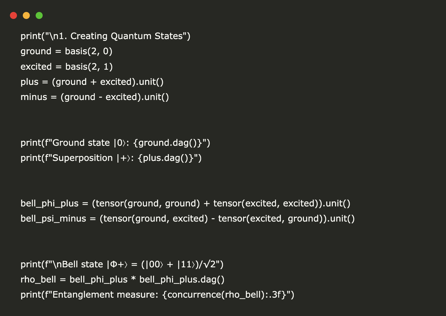
print("\n1. Creating Quantum States")
ground = basis(2, 0)
excited = basis(2, 1)
plus = (ground + excited).unit()
minus = (ground - excited).unit()


print(f"Ground state |0⟩: {ground.dag()}")
print(f"Superposition |+⟩: {plus.dag()}")


bell_phi_plus = (tensor(ground, ground) + tensor(excited, excited)).unit()
bell_psi_minus = (tensor(ground, excited) - tensor(excited, ground)).unit()


print(f"\nBell state |Φ+⟩ = (|00⟩ + |11⟩)/√2")
rho_bell = bell_phi_plus * bell_phi_plus.dag()
print(f"Entanglement measure: {concurrence(rho_bell):.3f}")
We begin by defining the computational basis states |0⟩ and |1⟩ and constructing their superpositions |+⟩ and |–⟩ to illustrate basic qubit manipulations. We then create Bell states to demonstrate maximal entanglement, computing their concurrence to quantify the entanglement. Check out the FULL CODES here.
print("\n2. Quantum Gates and Operations")
sx, sy, sz = sigmax(), sigmay(), sigmaz()
print(f"Pauli-X matrix:\n{sx}")


hadamard = (sx + sz) / np.sqrt(2)
cnot = tensor(fock_dm(2, 0), qeye(2)) + tensor(fock_dm(2, 1), sx)


h_ground = hadamard * ground
print(f"\nH|0⟩ = {h_ground.dag()}")
We explore the Pauli operators σₓ, σᵧ, and σ_z as the fundamental building blocks of qubit rotations and reflections. Using these, we construct the Hadamard gate for superposition generation and the CNOT gate for entangling operations, applying them to our prepared states. Check out the FULL CODES here.
print("\n3. Quantum Dynamics: Rabi Oscillations")
omega_0 = 1.0
omega_r = 0.5


H = 0.5 * omega_0 * sz + 0.5 * omega_r * sx


t_list = np.linspace(0, 4*np.pi/omega_r, 100)
psi0 = ground
result = mesolve(H, psi0, t_list, [], [])


excited_pop = [expect(fock_dm(2, 1), state) for state in result.states]


plt.figure(figsize=(12, 4))
plt.subplot(1, 2, 1)
plt.plot(t_list, excited_pop, 'b-', linewidth=2)
plt.xlabel('Time (ℏ/ω)')
plt.ylabel('Excited State Population')
plt.title('Rabi Oscillations')
plt.grid(True, alpha=0.3)
We model a driven two-level system with a Hamiltonian that couples σ_z and σₓ terms to simulate Rabi oscillations. By time-evolving the ground state under this Hamiltonian, we track the excited-state population oscillations and visualize them over a full Rabi cycle. Check out the FULL CODES here.
print("\n4. Quantum Harmonic Oscillator")
N = 20
a = destroy(N)
H_ho = a.dag() * a + 0.5


alpha = 2.0
psi0_coh = coherent(N, alpha)


t_list_ho = np.linspace(0, 2*np.pi, 50)
result_ho = mesolve(H_ho, psi0_coh, t_list_ho, [], [])


x_op = (a + a.dag()) / np.sqrt(2)
p_op = 1j * (a.dag() - a) / np.sqrt(2)


x_expect = [expect(x_op, state) for state in result_ho.states]
p_expect = [expect(p_op, state) for state in result_ho.states]


plt.subplot(1, 2, 2)
plt.plot(x_expect, p_expect, 'r-', linewidth=2)
plt.plot(x_expect[0], p_expect[0], 'go', markersize=8, label="Start")
plt.plot(x_expect[-1], p_expect[-1], 'ro', markersize=8, label="End")
plt.xlabel('⟨x⟩')
plt.ylabel('⟨p⟩')
plt.title('Coherent State Phase Space')
plt.legend()
plt.grid(True, alpha=0.3)
plt.axis('equal')


plt.tight_layout()
plt.show()
We extend our study to an N-level harmonic oscillator, initializing a coherent state and evolving it under the standard Hamiltonian. We compute and plot the phase-space trajectory ⟨x⟩ vs. ⟨p⟩ to observe classical-like motion in the quantum regime. Check out the FULL CODES here.
print("\n5. Quantum Decoherence and Open Systems")
gamma = 0.2
n_th = 0.1


c_ops = [np.sqrt(gamma * (1 + n_th)) * a, np.sqrt(gamma * n_th) * a.dag()]


psi0_sq = squeeze(N, 0.5) * basis(N, 0)


t_list_damp = np.linspace(0, 10, 100)
result_damp = mesolve(H_ho, psi0_sq, t_list_damp, c_ops, [])


n_expect = [expect(a.dag() * a, state) for state in result_damp.states]


plt.figure(figsize=(10, 4))
plt.subplot(1, 2, 1)
plt.plot(t_list_damp, n_expect, 'g-', linewidth=2)
plt.xlabel('Time')
plt.ylabel('⟨n⟩')
plt.title('Photon Number Decay')
plt.grid(True, alpha=0.3)
We introduce dissipation via collapse operators for a damped harmonic oscillator, simulating interaction with a thermal environment. We then evolve an initial squeezed state and monitor the decay of photon number ⟨n⟩ to illustrate decoherence effects. Check out the FULL CODES here.
print("\n6. Wigner Function Visualization")
final_state = result_damp.states[-1]
xvec = np.linspace(-4, 4, 50)
W_final = wigner(final_state, xvec, xvec)


plt.subplot(1, 2, 2)
plt.contourf(xvec, xvec, W_final, 20, cmap='RdBu')
plt.colorbar(label="W(x,p)")
plt.xlabel('x')
plt.ylabel('p')
plt.title('Wigner Function (Final State)')


plt.tight_layout()
plt.show()
We compute the Wigner quasi-probability distribution of the final damped state on a grid in phase space. By contour-plotting W(x,p), we gain intuitive insight into nonclassical features and the effect of decoherence on state coherence. Check out the FULL CODES here.
print("\n7. Entanglement Dynamics")
omega1, omega2 = 1.0, 1.1
g = 0.1


H_coupled = (omega1/2 * tensor(sz, qeye(2)) +
            omega2/2 * tensor(qeye(2), sz) +
            g * tensor(sx, sx))


psi0_prod = tensor(plus, ground)


t_list_ent = np.linspace(0, 20, 200)
result_ent = mesolve(H_coupled, psi0_prod, t_list_ent, [], [])


entanglement = [concurrence(state * state.dag()) for state in result_ent.states]


plt.figure(figsize=(8, 5))
plt.plot(t_list_ent, entanglement, 'purple', linewidth=2)
plt.xlabel('Time')
plt.ylabel('Concurrence')
plt.title('Entanglement Generation in Coupled Qubits')
plt.grid(True, alpha=0.3)
plt.ylim(0, 1)
plt.show()
We couple two qubits with a σₓ⊗σₓ interaction and evolve an initial product state, measuring concurrence at each time step. This allows us to observe the real-time buildup and decay of entanglement as a function of coupling strength and detuning. Check out the FULL CODES here.
print("\n8. Summary of Advanced Features Demonstrated:")
print("✓ Quantum state preparation and manipulation")
print("✓ Time evolution with mesolve()")
print("✓ Rabi oscillations in two-level systems")
print("✓ Coherent states and harmonic oscillators")
print("✓ Open quantum systems with decoherence")
print("✓ Wigner function visualization")
print("✓ Entanglement quantification and dynamics")


print(f"\n🎯 Tutorial complete! Explored {len(t_list_ent)} time steps")
print("Try modifying parameters to explore different quantum phenomena!")


print("\n💡 Advanced Exercises:")
print("1. Implement quantum error correction codes")
print("2. Simulate quantum algorithms (Grover, Shor)")
print("3. Explore cavity QED with Jaynes-Cummings model")
print("4. Study quantum phase transitions")
print("5. Implement quantum feedback control")
We recap the key demonstrations, state preparation, gate operations, time evolution, decoherence modeling, phase-space visualization, and entanglement quantification, and highlight how QuTiP’s mesolve() and built-in functions streamline these workflows. We conclude with suggestions for advanced exercises to deepen our exploration of quantum phenomena.
In conclusion, we’ve gone through the cornerstone phenomena of quantum mechanics, from superposition and entanglement to decoherence and phase-space visualization, using QuTiP’s intuitive API. Along the way, we prepared quantum states, applied gates, solved time-dependent dynamics with mesolve(), and quantified entanglement with concurrence. Our coherent-state and damped-oscillator examples revealed classical analogues in quantum phase space, while the coupled-qubit simulation showcased real-time entanglement growth. We encourage you to tweak parameters, such as coupling strengths, damping rates, and initial states, to deepen your understanding.
Check out the FULL CODES here. Feel free to check out our GitHub Page for Tutorials, Codes and Notebooks. Also, feel free to follow us on Twitter and don’t forget to join our 100k+ ML SubReddit and Subscribe to our Newsletter.
Sana Hassan, a consulting intern at Marktechpost and dual-degree student at IIT Madras, is passionate about applying technology and AI to address real-world challenges. With a keen interest in solving practical problems, he brings a fresh perspective to the intersection of AI and real-life solutions.
Credit: Source link